Collaborative Effort to predict hourly temperature drop during the August, 2017 Total Solar Eclipse

A total solar eclipse is a rare event. In the past 50 years, there has been only 1 total eclipse visible from the Southeast United States, on March 7, 1970, and just a handful of partial eclipses including May 30, 1984 which was a nearly total annular eclipse. Although these events are rare, many phenomena associated with them, including birds roosting, crickets chirping, stars and planets becoming visible, and even the elusive shadow bands, are well documented. For these reasons, the total solar eclipse on August 21, 2017 was a highly anticipated event across the entire continental United States.

This total solar eclipse was also exciting for the meteorological community. It is well known that temperatures cool during, and just after, a total solar eclipse, but the amount of cooling is quite uncertain. Leading up to the eclipse, examples of cooling from total solar eclipses in Zambia in 2001, and South Carolina in 1900, were referenced as possible analogs to what could be expected in 2017. The Zambia case was most widely distributed due to the observations of 15 degrees of cooling during that event, which led to extremely high forecasts of potential temperature drops of up to 20 degrees being predicted across social media and news outlets leading up to the 2017 event.

Temperature_change_1

Temperature curve from the 2001 total eclipse in Zambia. (https://eclipse2017.nasa.gov/temperature-change-during-totality)

The truth is that while some cooling was nearly certain, the amount of temperature drop was unknown. The National Weather Service (NWS) creates hourly temperature forecasts out through a 7 day forecast period twice a day, every day of the year, and in order to create an accurate forecast for the day of the eclipse, NWS offices would need to add some amount of cooling during the afternoon of August 21 to their hourly temperature forecasts. With such a high profile event, consistency and accuracy among NWS Weather Forecast Offices (WFO) was very important.

Realizing the need for a consistent prediction of temperature cooling during the eclipse, Josh Weiss from NWS Wilmington, NC developed an algorithm to reduce hourly temperatures based off data from the 1970 total and 1984 annular eclipses. METARs from 15 regional ASOS stations during the two eclipses were examined to analyze the temperature curves, cloud cover, and the solar obscuration percentage within a few hours of maximum eclipse. While this gave a nice picture of the hourly drop in temperature at each station, it didn’t truly solve the problem of the total drop from the typical diurnal temperature curve which is more important than the cooling from hour-to-hour. The NWS forecasts a diurnal curve in the hourly forecast, so determining the difference between the “expected” diurnal temperature and the actual temperature was the important parameter to determine.

Knowing this, a typical diurnal curve was then calculated for each station utilizing METAR data from the same calendar day from 6 prior years within the normal climate period (1981-2010), similar to the analysis done during the 1900 eclipse. From these curves, the difference between the realized temperature during maximum eclipse, and the expected temperature at that time on a typical diurnal day was calculated, and called diurnal drop. This was calculated for h(0) (hour closest to maximum eclipse) as well as h-1 and h+1.

1900duiurnalcurve

Temperature curves during the 1900 Total Solar Eclipse. Taken from 1902 U.S. Weather Bureau Report (https://www.ncei.noaa.gov/news/1900-total-solar-eclipse)

After completing this analysis, it was discovered that peak cooling occurred shortly after maximum eclipse, but that cloud cover played a much stronger role in determining diurnal drop than did solar obscuration. However, the variety of values was still not enough to determine if this was an accurate analysis of diurnal drop without some baseline value.

To solve this problem, the results of the analysis were compared to the NASA theory that states: The maximum temperature drop during a total solar eclipse can range from between ½ and ¾ the average diurnal range for the day (https://eclipse2017.nasa.gov/faq).

It is likely that the ¾ range would be for longer eclipses (a total solar eclipse can last up to 7 minutes) so with totality during the August 21 eclipse only lasting 2-3 minutes, the ½ value was used as a proxy for maximum potential drop during the event. This approach is quite helpful because utilizing this range will factor in time of year and humidity since the typical diurnal range in the Southeast during humid summer months can be smaller than during the cool and dry fall/winter months.

Putting all this together, an algorithm was developed to calculate expected maximum diurnal drop. The calculation included all the data from the previous eclipses, but also factored in a subtle difference for locations that would experience totality versus those that would not. This was included thanks to input from Frank Alsheimer at WFO CAE who provided guidance on local climatology and data from past eclipse events across Europe.

Maximum diurnal drop equation for solar obscuration = 100% at h(0):

If Sky Cover ≤ 50%:
Diurnal drop = 0.74 * ( ½ diurnal range)

If Sky Cover > 50% and Sky Cover ≤ 87%:
Diurnal drop = 0.64 * ( ½ diurnal range)

If Sky Cover > 87%:
Diurnal drop = 0.54 * ( ½ diurnal range)

For solar obscuration ≥ 90% but < 100% at h(0), the coefficients were reduced to 0.69, 0.59, and 0.49, respectively. A similar equation was developed for the h-1 and h+1 temperature changes, but the data was much more variable so that equation is not included here and instead saved for a more in depth study.

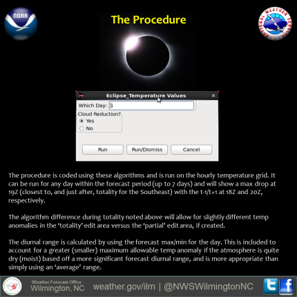
These calculations were then incorporated into a GFE smartTool and Procedure to provide the most scientifically sound and consistent method to adjust the hourly temperature forecasts. The tool would adjust the initial hourly temperature forecast during the period of the eclipse (17Z-20Z) with an eclipse based adjustment that includes forecast cloud cover and the percent of solar obscuration.

Eclipse GUI

GFE SmartTool interface used by forecasters

Once testing was completed, WFO ILM shared the GFE smartTool and Procedure with all the southeast WFOs hoping to create the most consistent and accurate forecast possible. Of these, 5 WFOs incorporated the tools into their GFE to create forecasts during the week leading up to the eclipse. Additionally, shapefiles of eclipse information were developed for use in some applications, GIS maps detailing eclipse obscuration percentages were installed in AWIPS, and methodologies and strategies were shared amongst the Southeast WFOs via a Google document.

jbmap

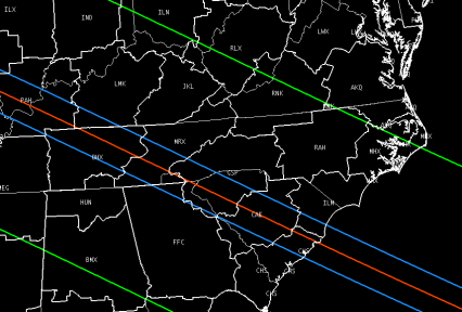
Map of the percentage of sun obscuration during the eclipse shown in AWIPS. The green lines are 90% or greater, the blue lines represent the path of totality, or 100%, and the red is the center line, or max totality.

The effort did not go unnoticed. Social media and news outlets began to note the forecast cooling created in both the NWS hourly weather graph as well as NDFD grid images as early as August 17th. The interest continued to ramp up through August 21st, with numerous posts made about NWS temperatures during the eclipse across all social media platforms.

Capturesmpost

Having a sound methodology among WFOs proved extremely beneficial, and with potentially millions of people heading to the Southeast for the eclipse it was crucial to have a consistent message from the local WFOs. This effort built on the history and relationships already in place across the CIMMSE domain, and is a great example of many NWS meteorologists and WFOs working together to provide enhanced forecasts and service.

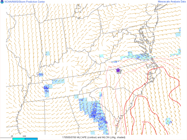
The weather pattern during the afternoon of August 21, 2017 featured an elongated ridge of high pressure aloft extending from the sub-tropical Atlantic westward across the Southeast into the Mississippi Valley.  A ridge of surface high pressure extended from off the Mid-Atlantic coast westward into the southern Appalachians. To the south, a decaying stationary surface boundary extended east to west from just off the North Carolina coast westward to the South Carolina coast and into southern Georgia. The air mass across the Southeast was generally weakly unstable although an axis of moderate instability, with mixed-layer CAPE values of 1500 J/Kg or more extended in an arc near the surface boundary west and northwest across the western Carolinas into the southern Appalachians.

Regions of enhanced cloudiness along with scattered convection developed during the early and mid-afternoon hours near and just off of the North Carolina coast and across much of coastal South Carolina in a region of greater moisture and instability and convergence near the surface boundary. More scattered cloudiness and isolated convection was noted across the remainder of South Carolina, western North Carolina, and especially across the higher terrain of the southern Appalachians. This cloudiness was associated with a weak shear axis aloft and enhanced by differential heating in the mountains. Elsewhere across the Southeast, skies were generally partly to mostly clear.

satellite

GOES-16 Channel 2 visible satellite imagery at 1822Z, just prior to totality in the Carolinas. Note the enhanced cumulus along the Appalachians, widespread cloud cover along the GA/SC/NC coasts, as well as the very dark area across TN/KY/MO which is beneath the totality shadow.

radar

Regional radar mosaic at 1848Z, during totality across SC. Rain and thunderstorms heavily impacted viewing along the coast as well as in a few locations in NC.

A forecast is only as good as its verification, and an after-event analysis was completed on 16 Southeast ASOS sites. The verification consisted of analyzing 1 minute temperature data for each site from NCDC and comparing the drop to the expected temperature value at that time. Data was acquired here:
(ftp://ftp.ncdc.noaa.gov/pub/data/asos-onemin/6406-2017)

To compare the algorithm performance to observations, METARs were examined for each of the 16 sites to acquire the max and min temperature for the day, as well as cloud cover during the eclipse, since this was not available in the minute data from NCDC. The algorithm was then applied to each site using the max/min as a proxy for the “expected” diurnal range and cloud cover, to produce the “forecast” diurnal drop. This value is what the algorithm would have given had the forecast of temperature and sky cover been correct; a perfect hindcast. Using this value as the forecast diurnal drop and comparing to the observed drop, provided the comparison for tool verification.

Of the 16 sites analyzed, 4 (CRE, CHS, GSO, INT) had to be removed due to precipitation or nearby convection and outflow affecting the temperature during the hours of the eclipse. Of the other 12, 5 had a perfect (0 degree error) forecast of diurnal drop, while 11 in total, or 92%, had measured diurnal drops within 2 degrees of the algorithm forecast. The last location (CAE) showed an error of just 3 degrees, just outside the acceptable “correct” forecast range.

finaleclipsedata_blog

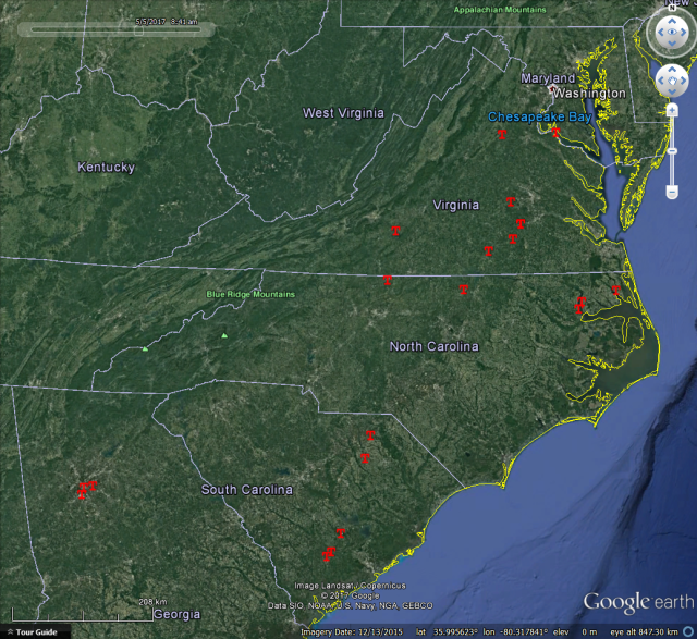
Results from the analysis. Locations in red were removed due to weather.

Verification so far has been excellent, but further work is needed. Analysis of all Southeast ASOS where solar obscuration was 90% or greater will be completed to further refine the results and ensure the accuracy of the algorithm. Once this is completed, it will be important to delve into the missed cases (error > 2 degrees) to try to determine why this occurred. Obtaining 1 minute cloud cover, if available, would supplement this study well.

Additionally, this algorithm was not the only one used to forecast temperature cooling across the country during the eclipse, and comparison to some of the other tools would be an interesting addition to this research. Perhaps a more nationally consistent methodology can be derived from this extended investigation, such that high confidence in diurnal cooling can be applied to hourly temperature curves during the 2024 total solar eclipse.

Many thanks to Jonathan Blaes at WFO RAH for his support and additions to this blog entry, and to Donald Hawkins at WFO ILM for a thorough and helpful review before publishing.

Posted in CIMMSE, Uncategorized | Leave a comment

Increasing Threat for HSLC Severe Weather on Tuesday Morning across Portions of Virginia and North Carolina

A quick look at some of the forecast products on the NC State HLSC web page suggests an increasing threat for severe weather on Tuesday morning. While the overall thermodynamic environment appears marginal, recent forecast trends suggest boundary layer moisture and instability will be a little greater than previously expected. Atop the increasing moisture, low and mid-level flow at 50-70kts will result in a strong warm advection pattern and shear.

SPC HREF surface based CAPE forecast postage stamps from the 01/22 12 UTC cycle valid at 15 UTC on Tuesday 01/23 shown below indicate only weak instability across eastern NC and eastern VA.

sbcape_ps.ma.f02700

At the same time, the 01/22 18 UTC cycle of the NAM valid at 15 UTC on Tuesday 01/23 shown below highlights northern and northeast NC and especially central and eastern VA for potential severe weather. At 15 UTC, the experimental SHERB and Modified SHERB composite parameters exceed 1 in this region suggestion the potential for HSLC significant severe reports. An introduction to the SHERB is available in this PDF: https://cimmse.wordpress.com/wp-content/uploads/2016/09/sherb.pdf

20180122.18z.f21

As a reminder, forecasts of the SHERB/SHERBE and the MOSH/MOSHE products are available for GFS, NAM, and RAP:

GFS
NAM
RAP

In addition, SPC mesoanalysis products for the Mid-Atlantic/Ohio Valley are available for the:
SHERBS3
SHERBE
MOSHE

Finally, as a part of our ongoing efforts to assess and improve the SHERB indices, we ask operational forecasters to submit feedback on the performance of the SHERB and modified SHERB, for both HSLC events and null cases: https://www.meas.ncsu.edu/mdparker/sherb/feedback

Posted in Uncategorized | Leave a comment

HSLC Products and Feedback Form

Given that Friday has at least some low-end HSLC potential in the Southeastern U.S., I took the opportunity to update the HSLC products feedback form so that it now includes questions about the so-called Modified SHERB (MOSH) and SHERBE (MOSHE).  The link to the survey is:

https://www.meas.ncsu.edu/mdparker/sherb/feedback

We sincerely appreciate your comments and assessments!


Also, as a reminder, we now have the MOSH/MOSHE products available for GFS, NAM, and RAP:

http://storms.meas.ncsu.edu/users/mdparker/gfs/hslc.html

http://storms.meas.ncsu.edu/users/mdparker/nam/hslc.html

http://storms.meas.ncsu.edu/users/mdparker/rap/hslc.html

Finally, in case you haven’t spotted it, SPC now plots the MOSHE as a part of their mesoanalysis:

http://www.spc.noaa.gov/exper/mesoanalysis/s17/moshe/moshe.gif

Please note that I am not sure whether the possible issues with their calculation have been corrected yet.  But, it may still be useful for a qualitative assessment.

Good luck to all with the coming winter/spring HSLC window, and please let us know if we can help!

Posted in Uncategorized | Leave a comment

Winter 2017 Mid-Atlantic and Southeast Sub-regional SOO and Northwest Flow Project Virtual Workshop

On December 13, a winter weather oriented sub-regional SOO and Northwest Flow Project virtual workshop was held. The workshop was organized following the Spring 2017 CSTAR Workshop and Mid-Atlantic and Southeast Sub-regional SOO meeting held in Raleigh where participants suggested getting together later and sharing information related to the cool season. More than 2 dozen folks participated from 17 different locations including 10 different WFOs and 3 different universities.

The workshop featured 3 different talks covering NCEP models and winter precipitation, winter weather NWP and automated detection of mesoscale snowbands and finally Dual-Pol radar in winter weather operations. Slide decks and recorded videos of the presentations from the workshop are available via Google Drive.

Links to the specific presentation materials and videos are also available in the agenda listing below…

  • Geoff Manikin, EMC Precip Type, Snow Accumulation, and Upslope Winter Precip in NCEP Models (slides | recording)
  • Gary Lackmann and Jacob Radford, NC State – Winter Weather NWP, and Automated Detection of Mesoscale Snowbands (NWP slides | Banding slides | recording)
  • Matthew Elliott, SPC – Dual-Pol Radar in Winter Weather Operations (slides | recording)

In addition, a couple of web sites were highlighted during the presentations including…

Posted in Uncategorized | Leave a comment

Late Spring HSLC Tornadoes across the Carolinas and Virginia: 4-5 May 2017

In association with a high amplitude closed upper low over the Mississsippi Valley, and a retreating wedge front at the surface, a mainly late night outbreak of wind damage and tornadoes occurred in a classic high shear, low CAPE (HSLC) environment, beginning late evening on May 4 and lasting beyond 8am on May 5.  There were a few tornado reports earlier in the day farther south that may not have occurred technically in low enough shear to meet the original CSTAR-defined thresholds for SBCAPE and MLCAPE, but most if not all in northern SC, and all of NC and VA did. This review will just focus on a couple of these tornadoes that were rated EF1 and not on the EF0s or the numerous reports determined to be straight line winds.

Synoptic U/A maps:


Fig1

Fig 1. 500 hPa Hgt/Temp  0000 UTC 05 May 2017.

Fig2

Fig 2. 850 hPa Hgt/Temp/DewPt  0000 05 May 2017


Surface frontal and large scale radar evolution:

Fig3

Fig 3. WPC surface analysis and radar mosaic, 0000 UTC 05 May 2017.


Fig4

Fig 4. Same as Fig 3 but for 0900 UTC.

SPC summary of national severe reports:

Fig5a Fig5b

Fig. 5.  SPC reports from 1200 UTC 04 May 2017 – 1200 05 May 2017 (left); and same for 05 May – 06 May (right).


Tornadoes that occurred between 8pm (May 4) and 8am (May 5) almost all appeared to occur in HSLC environments based on the Sherbun and Parker (2014) definition (SBCAPE of 500 J/kg or less, MUCAPE of 1000 J/kg or less, and 0-6km bulk wind difference of 18 ms-1 or more), when eyeballing the SPC mesoanalysis regional images.  Maps of the tornadoes (with all other reports removed) between 8pm – 8am are shown below.

Fig6

Fig. 6. All tornado reports between 0000 UTC (8pm) 04 May 2017 and 1200 UTC (8am) 05 May 2017.


Fig7

Fig. 7. Same as Fig 6 but zoomed in on northern NC and southeastern VA, and with the EF1 tornadoes highlighted along with time of touchdown and approx. path length labelled.


Following are some SPC mesoanalysis fields and radar images associated with the Rockingham Co NC EF1 at around 3am (the far SW tornado in Fig. 7 above):

Fig8

Fig. 8. MLCAPE at 0700 UTC 05 May 2017. Approximate location of Rockingham Co NC EF1 indicated by purple star.


Fig9

Fig. 9. Same as above but with 0-6km Bulk Shear Vector and magnitude.


Fig10

Fig. 10. Same as above but for 0-1km Storm Relative Helicity (SRH).


Fig11

Fig. 11. Same as above but for Sig Tor Parameter (STP).


Fig12

Fig. 12. Same as above but for SHERBE parameter.


Fig13

Fig. 13. Same as above but for Modified SHERBE (MOSHE).


Summarizing the above for the Rockingham Co NC EF1, the STP and SHERBE, while both showing underwhelming values in the location where the tornado occurred, at least indicated this was near the nose of a ridge for these parameters, but the MOSHE more clearly showed a maximum with values of at least 2.5.

Radar images for Rockingham Co NC EF1:


Fig14

Fig. 14. KFCX Z/SRM images at 0703 UTC (about 10 min before tornado touchdown) near Eden. Top images are the 0.5 deg slice, bottom ones are the 1.3 deg slice. Storm is about 45 nm from radar, and radar beam at 0.5 is about 6,000ft AGL. Radar is to the northwest.


Fig15

Fig. 15. Same as above but for 0711 UTC (about the time of touchdown near Eden).


Following are similar mesoanalysis fields as shown above but for 6am (was not able to capture 7am for most of these) and with the locations of the two Dinwiddie Co VA EF1s (a little south of Richmond) and the Orange Co VA EF1 (northeast of Charlottesville).


Fig16

Fig 16. MLCAPE at 1000 UTC (6am) May 05 2017. Approximate location of the two Dinwiddie Co EF1s (southern-most purple star) and of the Orange Co VA EF1 (northern-most purple star).


Fig17

Fig. 17. Same as above but for 0-1km SRH.


Fig18

Fig. 18. Same as above but for STP.


Fig19

Fig. 19. Same as above but for SHERBE.


Fig20a

Fig 20a. Same as above but for MOSHE.

Fig20b

Fig 20b. Same as above but for 1100 UTC (7am). [For some reason this was available at 7am but none the other fields were.]


Radar from Dinwiddie Co VA storm that produced two EF1 touchdowns, these are associated with initial touchdown. Radar configuration suggests more of a bow echo with circulation near comma head of bow, which was a common storm mode/configuration for several of the other tornadoes early this morning.


Fig21

Fig. 21. KAKQ radar at 1045 UTC, about 6 min before EF1 showing circulation coincident with comma-head region of bow echo. This location is just under 40nm from radar. Upper left panel is 0.5 deg, upper right 0.5 SRM, lower right is 0.5 NROT, and lower left is 1.3 Z.  


Fig22

Fig. 22. Same as above but at 1051 UTC (right at time of tornado touchdown), and lower left image is now CC showing subtle tornado debris signature (just to the left of the “M” in McKenney).

Note that a second tornado (also EF1) touched down in northern Dinwiddie Co. less than 20 min later with the same storm, and this was just after the bow echo signature went through a “Broken-S” evolution, the circulation briefly tightened again, and another TDS was observed as well (not shown).


Conclusions:

This is just a sampling of a few of the tornadoes associated with a classic High Shear Low CAPE (HSLC) environment, that were part of a nighttime outbreak of tornadoes and widespread severe weather on 4-5 May, 2017, and in association with a deep amplitude nearly vertically stacked upper-level trough and  retreating wedge front at the surface. Most of the tornadoes (if not all) that occurred between 8pm May 4 and 8am May 5 appeared to form in environments that easily fit the HSLC criteria from Sherbun and Parker (2014). A closer near-storm environmental analysis using surface observations and modified RAP soundings may be needed for each of these tornadoes in order to confirm this.

A closer look at the EF1 tornadoes in NC and VA showed that while they occurred on the northern edge of ridges in the analyses of traditional composite parameters (such as STP, and even the SHERBE), the Modified SHERBE (or MOSHE) seemed to show a better signal at the location of these tornadoes with values well above 1.0 in most cases. The caveat here is that the time shown for most of the analyses (1000 UTC) is about an hour before the tornadoes that are overlaid with them, but yet the 1100 UTC MOSHE analysis (which was available) fits pretty well with the tornadoes that occurred around that time.

Radar analysis of the storms associated with these tornadoes showed very shallow reflectivity signatures (and in fact, lightning activity was generally non-existent with them). In fact, in most cases there were only subtle signatures suggestive of a tornadic threat , such as small-scale bow echoes and in one or two cases evolving through “Broken-S” signature. Velocity fields did show weak to moderate circulations with many storms before the tornadoes touched down, but including some storms that did not produce known tornadoes.  Many of the tornadic storms were within 30-40nm of the nearest radar, but even so these signatures were often subtle, especially in terms of reflectivity structures.


Posted in Uncategorized | 3 Comments

Modified SHERB forecast plots now available

Forecast graphics for the modified SHERB (MOSH) and SHERBE (MOSHE) parameters are now available at the following links for the RAP, NAM, and GFS:

http://storms.meas.ncsu.edu/users/mdparker/rap/hslc.html
http://storms.meas.ncsu.edu/users/mdparker/nam/hslc.html
http://storms.meas.ncsu.edu/users/mdparker/gfs/hslc.html

shrbtiles.01.gif

Example 1-hour forecast RAP 4-panel of (top left) SHERBS3, (top right) SHERBE, (bottom left) MOSH, and (bottom right) MOSHE, valid 13Z 25 August 2017.

We have noticed that the calculated values show relative consistency between models, and the spatial footprints of enhanced values tend to be similar to those of the SPC Mesoanalysis. However, the values on the SPC Mesoanalysis are generally higher than those that we have calculated, again suggesting that there may be some discrepancies in the way SPC is calculating the parameters. I plan to touch base with SPC soon to ask about their progress on calculating individual terms of the MOSH/E parameters in order to determine where the differences arise.

Please feel free to utilize these plots as we transition into the HSLC season and share any insights you have!

Posted in Uncategorized | 2 Comments

Collaborative Effort to Account for the Impact of the August 21st Solar Eclipse on Operational Forecasts in the Mid Atlantic and Southeast

Map of the percentage of sun obscuration during the eclipse shown in AWIPS.

Map of the percentage of sun obscuration during the eclipse shown in AWIPS.

Meteorologists recognize that solar eclipses in the past have had a notable impact on the sensible weather in the regions in which they occur. These impacts can include a decrease in surface temperature, reduction and changes to surface winds, lowering of surface pressure, changes in cloud cover and more. National Weather Service (NWS) meteorologist in the Southeast and mid-Atlantic have been working collaboratively to account for some of these impacts on official NWS forecasts during the eclipse on Monday, August 21, 2017.

eclipse temp training

Image highlighting the some details of the Eclipse Temperature smartTool and Procedure for GFE.

Surprisingly, most operational numerical weather prediction (NWP) systems do not account for the changes in incoming solar radiation from the sun during an eclipse and the resultant changes in the weather. This is an issue as NWS forecasters provide forecasts of temperature, winds, and other fields at hourly time steps and the eclipse impacts need to be captured by forecaster intervention over model guidance. The effort to provide details on the eclipse impact on weather in our region began with the development of hourly temperature reductions based on past eclipse events and factoring local climatology proposed by Frank Alsheimer at WFO CAE. Additional WFOs in the CIMMSE area collaborated and provided input on reductions while working within the temporal confines of the National Digital Forecast Database. Joshua Weiss at WFO ILM, examined data from the 1970 and 1984 eclipses in the Southeast and created a GFE smartTool and Procedure to provide a more scientifically sound and consistent process to edit the hourly temperature forecasts.

meteograms

Official hourly forecasts of temperature and sky cover from three locations in adjacent WFOs CAE, ILM, and RAH. The temperatures were adjusted using the Eclipse Temperature GFE procedure. Columbia, SC is in the eclipse totality while Lumberton, NC and Wadesboro, NC reach 97% obscuration. Differing temperature reductions during and after the eclipse are influenced by various factors including differing amounts of cloud cover.

The GFE Procedure incorporates the forecast temperature and diurnal range without the eclipse impact, whether a location is in the total or partial eclipse, and the amount of cloud cover. Nearly a half dozen WFOs in the Southeast will be using this tool which should lead to a more consistent, more scientifically sound, and accurate forecast. In addition, shapefiles of eclipse information were developed for use in some applications, GIS maps detailing eclipse obscuration percentages were installed in AWIPS, and finally methodologies and strategies were shared via a Google document. This effort builds on the history and relationships built across the CIMMSE domain. The event is a great example of many NWS meteorologists and WFOs working together to provide enhanced forecasts and service.

hrrx.example

Screen shot of the High-Resolution Rapid Refresh (HRRRx) experimental real-time weather forecast web page the eclipse.

It is also worth noting that some experimental and non-operational NWP systems will account for the eclipse. NOAA/ESRL/GSD made changes to the 3km experimental HRRR (HRRRx) to include code to account for the sun-obscuration from the eclipse (details… https://esrl.noaa.gov/gsd/learn/hotitems/2017/eclipse2017-hrrr.html). For real-time HRRRx experimental forecasts, including the effects of the eclipse starting Saturday night looking ahead 48 hours with the 00 UTC model run, visit https://eclipse2017.noaa.gov. Some of the selected weather fields available include downward solar radiation, cloud fields and 2-meter temperature, for the HRRRx (with eclipse effect), the operational HRRR-NCEP (without eclipse effects and some other differences) and HRRRx – HRRR-NCEP difference fields.

Posted in CIMMSE, NWP | Leave a comment

A pair of HSLC-related presentations: NOAA VLab Forum and AMS Mesoscale Conference

Over the last few months, I have provided two presentations on recent HSLC-related research. In June, I was the presenter at NOAA’s VLab Forum, where I provided an overview of the ongoing HSLC CSTAR project based at NC State University. A recording of this presentation can be found here.

The next month, I traveled to the AMS Conference on Mesoscale Processes in San Diego, where I presented an update on my ongoing idealized modeling work. Of particular interest, I have identified the chain of processes appearing to result in the development of strong, low-level vortices within simulated HSLC QLCSs and determined how low-level shear vector magnitude and low-level lapse rates could affect these processes.


Simulation-based research continues, and I intend to complete and defend my dissertation later this fall. Please let me know if you have any questions or comments!

Posted in CIMMSE, Convection, CSTAR, High Shear Low Cape Severe Wx | Leave a comment

Operational NWP Resolution and Sensitivities Study Using HSLC Event Hindcasts Summary

At last month’s CSTAR workshop, I shared the results and analysis of my thesis project as well as some thoughts on related future work. I would like to provide a summary of my and Dr. Lackmann’s work with this post for those who could not be there and as a refresher for those who were.

The problem I focused on is that severe convection that forms in  High Shear, Low CAPE (HSLC) environments is difficult to predict and is dangerous. There are two approaches to improve HSLC severe convection predictability: the first is the use of environmental predictors such as the SHERB (Sherburn and Parker 2014) and the MOSH (Sherburn et al. 2016) and the second is using Numerical Weather Prediction (NWP) models to predict convection which is what myself and Jessica King did (King et al. 2017). This research project sought to answer two research questions:

1. At what horizontal grid spacing, if any, does an NWP model provide operationally useful information about explicit low instability severe convection?
2. Can a NWP model properly differentiate between a HSLC event case and a HSLC null event case given the proper initial conditions?

Dr. Lackmann and I  looked at two cases, a event case February 24-25, 2011, a null case, December 25-26, 2009. I ran these cases using the WRF model at convection-permitting grid spacings (Figure 1) and then evaluated how well each domain represented the severe weather using severe proxy metrics: half-hourly maximum updraft helicity (1-4km), half-hourly maximum 10-meter wind speed, half-hourly maximum updraft speed, and composite radar reflectivity (Figure 2). In order to compare the different domains on an “equal playing field” so to speak, we conformed the 1.2-km and 400-m domains to a grid with a 3.6-km grid spacing over the area encompassed by the 400-m domain. The severe proxy metrics were calculated on the higher resolution domain first before this interpolation. This process is effectively sub-sampling. The distributions of the severe proxy values of these interpolated domains were compared to one another both in the same case and between the two cases (Figure 3).

The results of this analysis are as follows:
– Based on this study, the recommended horizontal grid spacing to run a NWP model in a way that provides operationally useful information about low instability convection is 3.6-km.
– A larger gain in detail is observed between the 3.6-km and 1.2-km domains than between the 1.2-km and 400-m domains.
– Overall, the event case and null event case are statistically significantly different. It is important to note that there is a difference between differentiating and distinguishing; the model had difficulty distinguishing between the two cases.
– Thresholds of severe proxy parameters, especially updraft helicity, should be adjusted to handle finer model resolution.

I look forward to receiving your questions and comments as well as participating in any discussion that follows. Please feel free to ask me questions in the comments section or to send an email to lrblank@ncsu.edu. Thank you!

modelconfig_02242011
Figure 1: Model domain set up for the event case February 24-25, 2011

02252011_03utc_refc_comp
Figure 2: NEXRAD and conformed model domain composite radar reflectivity for the event case. Time shown is 03:00 UTC on 02/25/2011.

eventvnull_uh
Figure 3: The severe proxy conformed half-hourly maximum updraft helicity distributions for the event case and null event case at each convective permitting domain.

References:

King, J.R., M.D. Parker, K.D. Sherburn, and G.M. Lackmann 2017: Rapid Evolution of Cool Season, Low CAPE Severe Thunderstorm Environments. Wea. Forecasting. doi: 10.1175/WAF-D-16-0141.1

Sherburn, K.D., and M.D. Parker, 2014: Climatology and Ingredients of Significant Severe Convection in High-Shear, Low-CAPE Environments. Wea. Forecasting, 29, 854-877, doi: 10.1175/WAF-D-13-00041.1

———-, ———–, G.M. Lackmann, and J.R. King, 2016: Composite environments of severe and non-severe high-shear, low-CAPE convective events. Wea. Forecasting. Doi: 1175/WAF-D-16-0086.1

Posted in CIMMSE, Convection, CSTAR, High Shear Low Cape Severe Wx, NWP, Uncategorized | Tagged , | Leave a comment

Updated List of NC State-NWS CSTAR Publications

King_Parker_CSTAR2017

Figure depicting the change in surface based CAPE in the hours prior to severe convection in HSLC environments as described in King et al., 2017.

Shown below is a list of publications and abstracts developed as a part of the most recent NC State-NWS CSTAR project entitled “Understanding and Prediction of High Impact Weather Associated with Low-Topped Severe Convection in the Southeastern U.S.” Note that additional presentations are scheduled for upcoming conferences including the AMS 24th Conference on Probability and Statistics in July and the 17th Conference on Mesoscale Processes in July. In addition, manuscripts are being composed for multiple projects including the predictability study using ensembles and dynamical-statistical downscaling project.

Publications (most recent first):

1) King, J. R., M. D. Parker, K. D. Sherburn, and G. M. Lackmann, 2017: Rapid evolution of cool season, low CAPE severe thunderstorm environments. Wea. Forecasting, 32, 763-779. | PDF |

2) Sherburn, K. D., M. D. Parker, J. R. King, and G. M. Lackmann, 2016: Composite environments of severe and non-severe high-shear, low-CAPE convective events. Wea. Forecasting, 31, 1899-1927. | PDF |

Conference abstracts (most recent first):

1) Sherburn, K. D., and M. D. Parker, 2016: The origins of rotation within high-shear, low-CAPE mesovortices and mesocyclones. 28th Conference on Severe Local Storms, AMS, 7-11 November 2016, Portland, OR. | Recorded presentation | Manuscript |

2) Sherburn, K. D., and M. D. Parker, 2016: Insights from composite environments of high-shear low-CAPE severe convection. 28th Conf. on Severe Local Storms, AMS, 7-11 November 2016, Portland, OR. | Poster handout | Manuscript |

3) Blank, L., and G. Lackmann, 2016: Operational predictability of explicit high shear, low CAPE convection. 6th Conference on Transition of Research to Operations, AMS, 11-14 January 2016, New Orleans, LA. | Recorded presentation |

4) King, J. R., and M. D. Parker, 2015: Conditioning and evolution of high shear, low CAPE severe environments. 16th Conference on Mesoscale Processes, AMS, 2-6 August 2015, Boston, MA. | Recorded presentation | Manuscript |

5) Sherburn, K. D., and M. D. Parker, 2015: Examining the sensitivities of high-shear low-CAPE convection to low-level hodograph shape. 16th Conference on Mesoscale Processes, AMS, 2-6 August 2015, Boston, MA. | Recorded presentation | Manuscript |

6) King, J. R., and M. D. Parker, 2014: Synoptic influence on high shear, low CAPE convective events. 27th Conference on Severe Local Storms, AMS, 2-7 November 2014, Madison, WI. | Poster handout | Manuscript |

7) Sherburn, K. D., and M. D. Parker, 2014: High-shear, low-CAPE environments: What we know and where to go next. 27th Conference on Severe Local Storms, AMS, 2-7 November 2014, Madison, WI. | Recorded presentation | Manuscript |

8) Sherburn, K. D., and M. D. Parker, 2014: On the usage of composite parameters in high-shear, low-CAPE environments. 27th Conference on Severe Local Storms, AMS, 2-7 November 2014, Madison, WI. | Poster handout | Manuscript |

Posted in Uncategorized | Leave a comment